Project 1 of my data analytics portfolio: a SQL and Tableau audit of delivery performance on a 100,000-order Brazilian e-commerce marketplace.

→ Live interactive dashboard on Tableau Public · Full SQL on GitHub

Nearly 1 in 3 sellers on this marketplace has shipped at least one late order. Sort them by average delivery delay, and you’d flag exactly the wrong people: a seller with a single 134-day disaster would outrank a seller who has been late over 100 different times. I built that ranking, trusted it for about five minutes, then had to go back and fix my own method once I saw who it was actually surfacing.

This is the full build, close to how it actually happened—the concepts as I learned them, the exact queries that failed and why, and the reasoning behind decisions that aren’t visible in the finished SQL alone.

Why this project?

⁣I picked Olist’s Brazilian E-Commerce Public Dataset for the project because it’s messy and close to real business data. What actually makes a portfolio project stand out is the business question, not whether the CSV is one nobody’s seen before. “Is this seller hurting our customers?” is a question any manager/owner understands immediately, in any industry.

Why SQL first, not Python? I could have run this in pandas. I did it in a live Postgres database instead (via Supabase, not a local file) because SQL is the most commonly screened-for skill and because most companies’ real data lives in a warehouse, not a CSV.

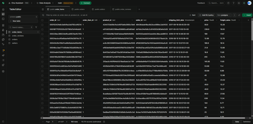
This dataset ships as nine relational CSVs. I only imported four: orders, order_items, sellers, and order_reviews. Deciding what’s out of scope before touching a database is its own skill; loading five tables I’d never query; it just adds noise.

The Analysis

Step 1: Delay at the order level

Every SQL query has three core pieces: SELECT (which columns), FROM (which table), and WHERE (which rows survive). Postgres lets you subtract two timestamps directly, and it hands back an interval, order_delivered_customer_date - order_estimated_delivery_date.

This returns something like 3 days 04:12:00. Positive means the order arrived after the estimate (late); negative means early.

The task I set out to solve: write a query against orders returning order_id, order_estimated_delivery_date, order_delivered_customer_date, via a computed column, “delay” showing that difference, filtered to delivered orders only, and sorted so the latest arrivals show up first.

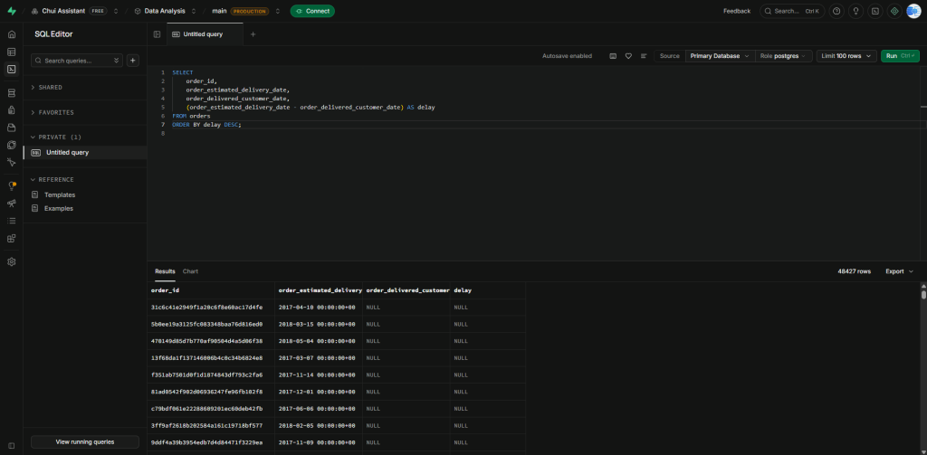
Attempt one:

SELECT order_id, order_estimated_delivery_date, order_delivered_customer_date,
    (order_estimated_delivery_date - order_delivered_customer_date) AS delay
FROM orders
ORDER BY delay DESC;

Two bugs. The subtraction is backwards, estimated - delivered giving a negative number when an order is late since “delivered” is the bigger value.

So ORDER BY delay DESC was surfacing my earliest deliveries, not my latest ones. Second, there’s no filter for undelivered orders, which have a NULL delivered date, and Postgres sorts NULL first in a DESC order by default, so the top of the results was a wall of nulls, not real data.

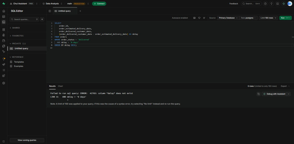
Attempt two: I flipped the subtraction and added order_status = 'delivered', both correct fixes, but introduced a new problem:

SELECT order_id, order_estimated_delivery_date, order_delivered_customer_date,
    (order_delivered_customer_date - order_estimated_delivery_date) AS delay
FROM orders
WHERE order_status = 'delivered'
  AND delay > '0 days'
ORDER BY delay DESC;

This throws column "delay" does not exist. SQL doesn’t execute top to bottom. The real order is FROM → WHERE → SELECT → ORDER BY.

The alias delay gets created at the SELECT step but WHERE runs before that, so as far as WHERE is concerned, delay column doesn’t exist yet. That’s also why ORDER BY delay works fine in both attempts and ORDER BY runs last.

Two ways around it: filter on the real columns instead of the alias (WHERE order_delivered_customer_date > order_estimated_delivery_date), or wrap the calculation in a CTE so the outer query treats delay as a genuine column.

I chose the CTE and kept using that pattern for the rest of the project. Once queries stack three or four transformations deep, having each step named and independently readable matters more than saving a couple of lines.

WITH delivery_delays AS (
    SELECT order_id, order_estimated_delivery_date, order_delivered_customer_date,
        (order_delivered_customer_date - order_estimated_delivery_date) AS delay
    FROM orders
    WHERE order_status = 'delivered'
)
SELECT * FROM delivery_delays
WHERE delay > interval '0 days'
ORDER BY delay DESC;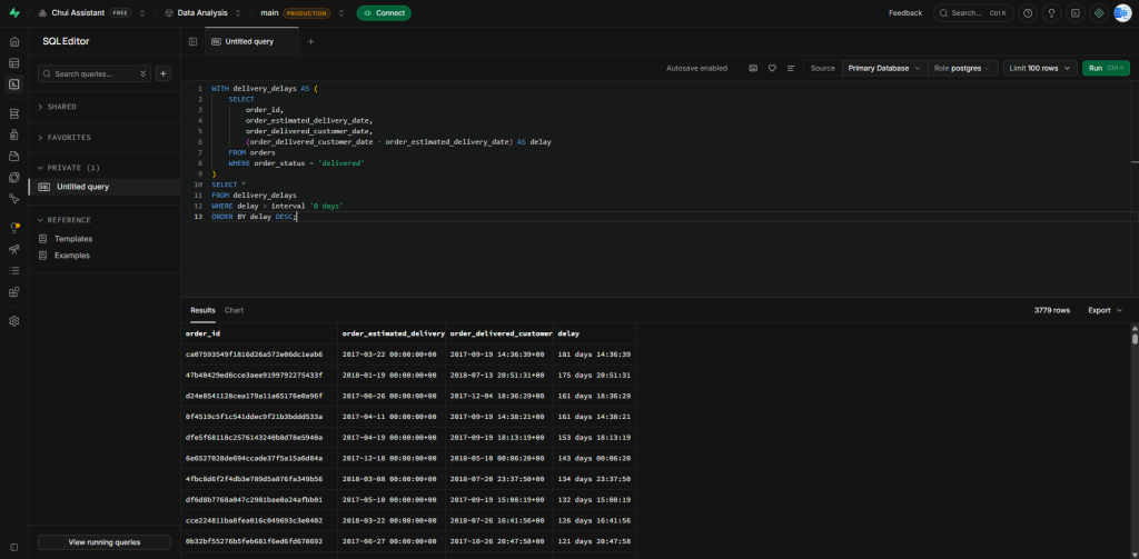

Timestamp error

If you run the SQL above, you might get an error: operator does not exist: text - timestamp with time zone (Didn’t get a screenshot). This means one of the two date columns hasn’t been imported as a real timestamp. It is sitting on the table as plain text. I checked with a query that became a standing habit for the rest of the project:

SELECT column_name, data_type
FROM information_schema.columns
WHERE table_name = 'orders'
ORDER BY ordinal_position;

Three columns had come in as text: order_approved_at, order_delivered_carrier_date, order_delivered_customer_date. The pattern was consistent.

These three can legitimately be blank (an order that’s never been delivered has no delivery date), while order_purchase_timestamp and order_estimated_delivery_date are always populated, and those two were imported correctly.

Supabase’s CSV auto-import couldn’t confidently infer a type when it encountered blank cells alongside valid dates, so it fell back to text for the entire column. Fixed once, for all three, at the schema level:

ALTER TABLE orders
  ALTER COLUMN order_approved_at TYPE timestamptz
    USING NULLIF(order_approved_at, '')::timestamptz,
  ALTER COLUMN order_delivered_carrier_date TYPE timestamptz
    USING NULLIF(order_delivered_carrier_date, '')::timestamptz,
  ALTER COLUMN order_delivered_customer_date TYPE timestamptz
    USING NULLIF(order_delivered_customer_date, '')::timestamptz;

NULLIF(column, '') Converts the empty-string blanks to a real NULL before the cast; skip that and the cast fails the moment it hits a blank row.

Given that bug existed in one table, I checked the other three (order_items, sellers, order_reviews) the same way before building anything on top of them.

All three came back clean, each for a specific, checkable reason: order_items‘s only date field (shipping_limit_date) gets set the instant an order is placed, so there’s no blank-cell scenario; sellers has no date columns at all; and order_reviews only has a row when a customer actually submitted a review, so there’s no such thing as a blank future review date the way there was a blank future delivery date.

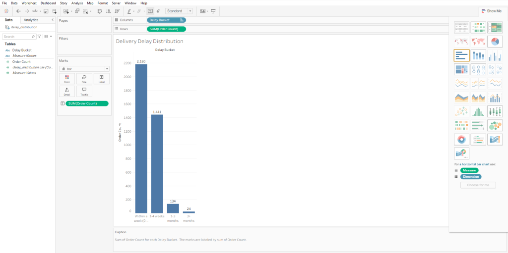
Finding: 3,779 delivered orders arrived late, with the single worst individual order at 181 days, a spike consistent with the Brazilian trucking strikes documented in this exact April 2017 and February–March 2018 window. The distribution is heavily right-skewed, which I confirmed with a conditional-aggregation pattern I hadn’t used before — COUNT(CASE WHEN condition THEN 1 END), which returns 1 per matching row and NULL, and COUNT quietly ignores the nulls:

SELECT
    COUNT(CASE WHEN delay <= interval '7 days' THEN 1 END) AS within_a_week,
    COUNT(CASE WHEN delay > interval '7 days' AND delay <= interval '30 days' THEN 1 END) AS one_to_four_weeks,
    COUNT(CASE WHEN delay > interval '30 days' AND delay <= interval '90 days' THEN 1 END) AS one_to_three_months,
    COUNT(CASE WHEN delay > interval '90 days' THEN 1 END) AS over_three_months
FROM delivery_delays;

57.7% of late orders ran under a week, 38.1% ran one to four weeks, 3.5% ran one to three months, and 0.6% (24 orders) ran past three months.

Step 2: From late orders to late sellers

seller_id lives on order_items, not orders, so this needed a join. JOIN ... ON matches rows wherever a condition holds, and both tables needed aliasing (o, oi) since both have a column called order_id.

Before writing anything, two things were worth flagging: a single order can contain items from more than one seller, so that order’s delay gets attributed to every seller involved; and order_items has one row per item, not per order, so a naive COUNT(*) after the join counts items, not orders.

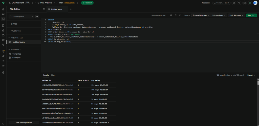
Attempt one ignored the second issue:

SELECT oi.seller_id, COUNT(o.order_id) AS late_orders,
    AVG(o.order_delivered_customer_date - o.order_estimated_delivery_date) AS avg_delay
FROM orders o
JOIN order_items oi ON o.order_id = oi.order_id
WHERE o.order_status = 'delivered'
  AND o.order_delivered_customer_date > o.order_estimated_delivery_date
GROUP BY oi.seller_id
ORDER BY avg_delay DESC;

COUNT(o.order_id) isn’t the same as COUNT(DISTINCT o.order_id), if a seller shipped 2 items on the same late order, that order gets counted twice.

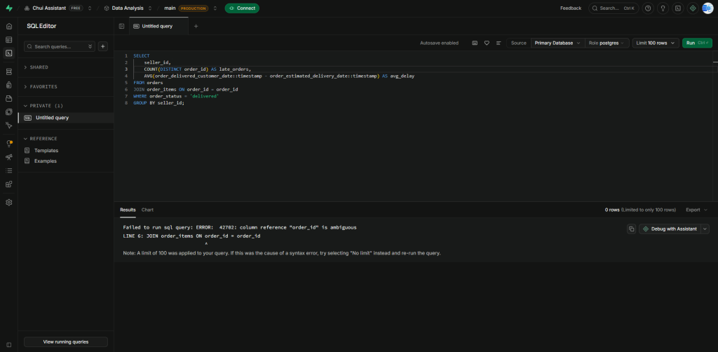
Attempt two: added DISTINCT to the count but wrote the join as ON order_id = order_id with no table prefix, which throws column reference "order_id" is ambiguous. Both tables have that column, and it also silently dropped the late-orders-only filter.

The deeper issue neither draft caught: AVG() has the exact same fan-out problem as COUNT(). Fixing the count with DISTINCT does nothing for the average, and a duplicated row still gets averaged in twice. The real fix is structural: deduplicate to one row per order-seller pair before aggregating anything, not after.

WITH order_delays AS (
    SELECT order_id, (order_delivered_customer_date - order_estimated_delivery_date) AS delay
    FROM orders
    WHERE order_status = 'delivered'
      AND order_delivered_customer_date > order_estimated_delivery_date
),
seller_order_delays AS (
    SELECT DISTINCT od.order_id, oi.seller_id, od.delay
    FROM order_delays od
    JOIN order_items oi ON od.order_id = oi.order_id
)
SELECT seller_id, COUNT(*) AS late_orders, AVG(delay) AS avg_delay
FROM seller_order_delays
GROUP BY seller_id
ORDER BY avg_delay DESC;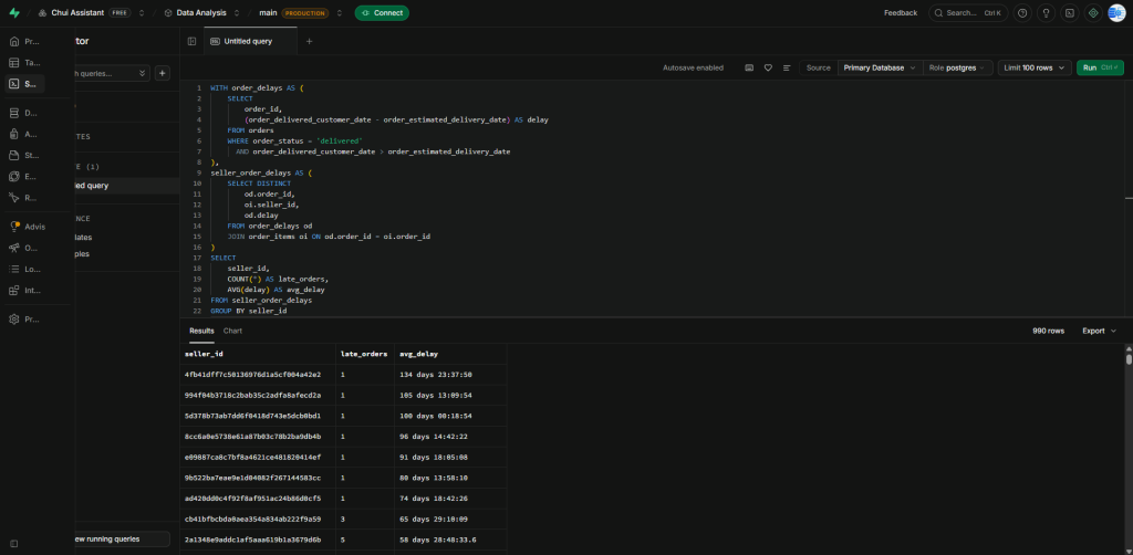

I ran a reconciliation check, not because I suspected an error. I wanted to compare Step 1’s 3,779 distinct late orders against the row count of seller_order_delays:

SELECT COUNT(DISTINCT seller_id) AS sellers_with_late_orders,
    COUNT(*) AS seller_order_pairs,
    (SELECT COUNT(*) FROM order_delays) AS distinct_late_orders,
    COUNT(*) - (SELECT COUNT(*) FROM order_delays) AS multi_seller_gap
FROM seller_order_delays;

That returned 3,790 seller-order pairs against 3,779 distinct orders, an 11-order gap. This is fully explained by the multi-seller caveat flagged before writing a line of code.

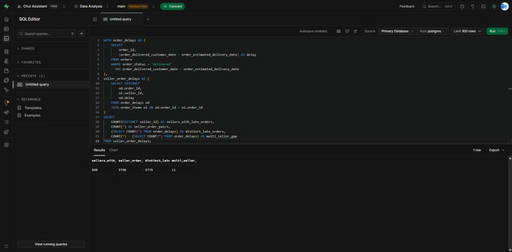
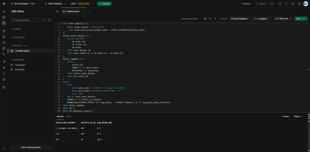
I also checked, with the same conditional-count pattern from Step 1, how late-order volume related to average delay, bucketing sellers into “1 incident,” “2–9,” and “10+” late orders and averaging delay within each bucket.

The 1-incident group had the worst-looking average by a wide margin, which is the first hint of the ranking problem in Step 3.

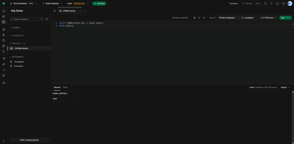
Finding: 990 of 3,095 sellers — 31.99% — have shipped at least one late order.

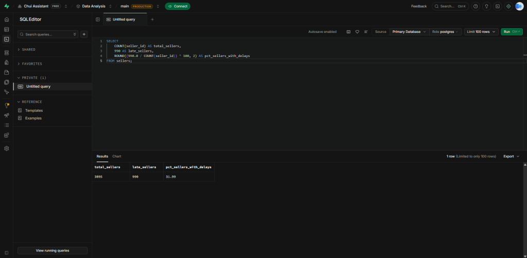
That percentage was first computed with the seller count hardcoded (990.0 / COUNT(seller_id)), which works but silently goes stale the next time the data refreshes. Fixed this with a subquery instead of a literal.

Step 3: Why “average delay” alone ranks the wrong sellers

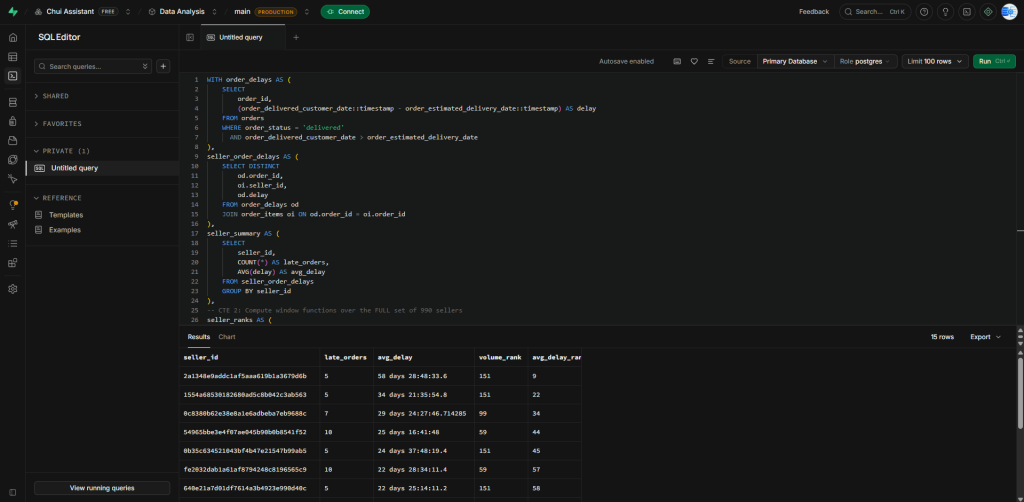
GROUP BY collapses rows into a summary; a window function keeps every row but adds a value computed across a related set. RANK() OVER (ORDER BY late_orders DESC) doesn’t group anything; every seller keeps their own row, but each one now also knows its rank relative to every other seller.

Sorting sellers by average delay puts one-time flukes at the top: a seller with a single catastrophic delay outranks a seller who has been late over 100 separate times because an average built from a sample of one isn’t really an average; it’s a single number wearing a disguise.

Before ranking, I set a threshold for at least 5 late orders over the full population of 990 sellers before any filtering. Filtering first and ranking second would have given me a rank relative to a pre-shrunk subset, not the true population.

seller_ranks AS (
    SELECT seller_id, late_orders, avg_delay,
        RANK() OVER (ORDER BY late_orders DESC) AS volume_rank,
        RANK() OVER (ORDER BY avg_delay DESC) AS avg_delay_rank
    FROM seller_summary
)
SELECT * FROM seller_ranks
WHERE late_orders >= 5
ORDER BY avg_delay_rank ASC
LIMIT 15;

The top 15 avg_delay_rank were all sellers with 5 to 12 late orders and 18–58 day averages. Every seller I’d previously flagged as a high-volume repeat offender was completely absent from this list.

RANK() Also tied correctly: five sellers tied at volume_rank = 151 (with exactly 5 late orders), and the next distinct rank jumped straight to 156.

Running the complementary query with the same CTEs, sorted by volume_rank Instead, no filter is needed since high-volume sellers already clear any reasonable threshold showed a completely different group: one seller with 102 late orders but only a 9.8-day average (#1 by volume, #303 out of 990 by average delay) and another with 82 orders and a similar mild average.

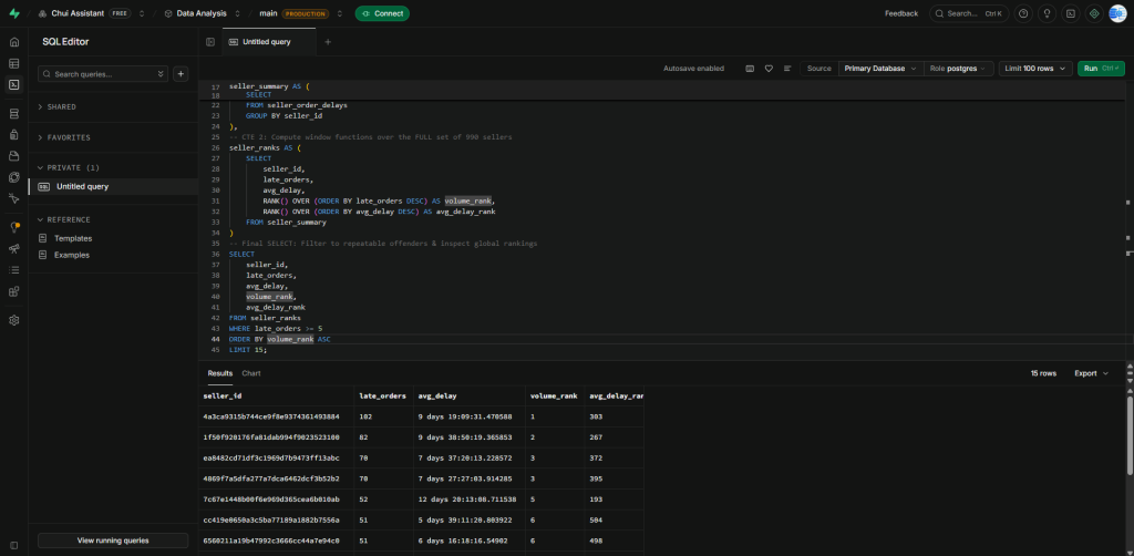
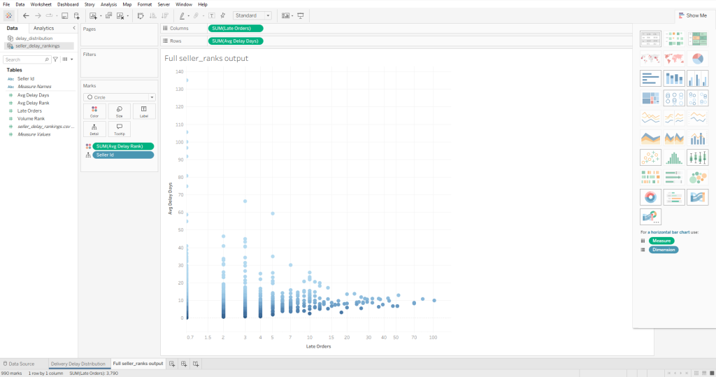
Two real, different failure patterns. I labeled them “severe-but-rare” and “frequent-but-mild,” but the scatter plot (Step 5) makes clear this is a simplification of something continuous, not two hard-edged clusters.

As a seller’s late-order count climbs, their average delay tightens sharply toward 7–12 days and essentially never revisits the extremes.

That’s the same reason a product with 10,000 reviews at 4.8 stars is more trustworthy than one with a single 5-star review: a seller needs nearly all of their late orders to be extreme for their average to stay extreme, which rarely happens once volume climbs.

Step 4: Does any of this actually cost the business anything?

Everything so far proves sellers are late. It doesn’t prove that it costs anything.

First, a handful of orders had two review rows instead of one (GROUP BY order_id HAVING COUNT(*) > 1 confirmed it); I deduplicated it the same way as Step 2, averaging review_score per order in a CTE before joining anything to it.

Second, why a LEFT JOIN, not an inner join? A share of delivered orders never got reviewed at all. An inner join would silently drop every one of them from the comparison. The numbers might still look fine, but there’d be no way to know how much data quietly vanished.

A LEFT JOIN, followed by an explicit WHERE review_score IS NOT NULL, keeps that exclusion visible: I could state exactly how many orders each average was built on (42,962 vs. 3,711) instead of just trusting it was enough.

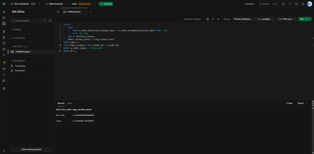
The CASE WHEN statement labeled orders as ‘Late’ or ‘On-Time’ by directly comparing two dates. However, in SQL, NULL > anything evaluates to NULL, causing the CASE WHEN to default to the ELSE branch if any ‘delivered’ order lacks a delivery date.

This means such orders could be incorrectly marked as ‘On-Time’ due to a lack of information. A quick check (COUNT(*) WHERE order_status = ‘delivered’ AND order_delivered_customer_date IS NULL) confirmed this issue, highlighting the importance of validating logic rather than assuming it’s error-free.

I created a seller_segments CTE based on the ranking CTEs from Step 3 and joined it with seller_order_delays to focus on each segmented seller’s late orders. A plain JOIN was appropriate since every seller in seller_segments is guaranteed to exist in seller_order_delays, making a LEFT JOIN unnecessary and misleading.

I expected severe-but-rare sellers to score worse than frequent-but-mild ones, as one dramatic delay leaves a stronger impression than several minor ones. The data supported this, showing 1.97 for severe-but-rare versus 2.49 for frequent-but-mild, though this is based on just 30 reviewed orders across 5 sellers, making it more of a lead than a definitive conclusion.

Both segment averages fell below the overall “Late” average of 2.57. This makes sense because the overall average includes all mildly-late sellers, while these segments represent the extremes, naturally scoring worse than the blended average.

Step 5: Building the dashboard

Tableau sorts categories alphabetically by default, which would have scrambled my delay-bucket chart’s story (fixed with a manual sort)

Tableau aggregates measures by default the same way SQL collapses rows without a GROUP BY, dragging my two seller-level measures onto the scatter plot’s axes produced exactly one dot until I told it to keep one mark per seller. Most sellers cluster at low volume, and the cloud narrows sharply as volume climbs.

The review score bar chart needed the same manual-sort fix as the first chart, arranged narratively (On-Time → Late → Frequent-but-mild → Severe-but-rare) instead of alphabetically.

Combining everything into one dashboard, I deliberately didn’t wire up cross-filtering between the three charts.

Thoughts

I started this project assuming that once I could calculate an average, I had my answer. An average is only as trustworthy as the sample behind it; once I saw a seller with 102 late orders sitting nowhere near the top of a list sorted by average delay.

I also started out treating my early bugs as things to quietly fix and move past. The reconciliation check between 3,779 and 3,790 is proof my hunch about multi-seller orders was actually correct.

The findings, stated plainly

• 31.99% of sellers have shipped at least one late order.
• Ranking by average delay alone hides the real problem: a seller with 102 late orders and a seller with 5 late orders can both look “not that bad” or “the worst,” depending entirely on which single number you sort by.
• Lateness is associated with a real, well-powered 1.73-star drop in average review score.
• Sellers who fail rarely but severely appear to hurt reviews more than sellers who fail constantly but mildly — though that specific comparison rests on a small sample and should be read as a lead, not a settled fact.

Two key limitations are: first, this is correlation, not causation; a late order may also arrive damaged or come from a problematic seller. Second, the two-segment framing simplifies a continuous relationship for actionable insights, rather than presenting just a raw scatter plot.

Close

The full interactive dashboard, including the scatter plot referenced throughout this post, is live on Tableau Public. The complete SQL and a more technical write-up are on GitHub.

If you’re hiring for an analyst or analytics engineering role, I’d like to hear about it.